Smith Chart and Matching Circuit Fundamentals
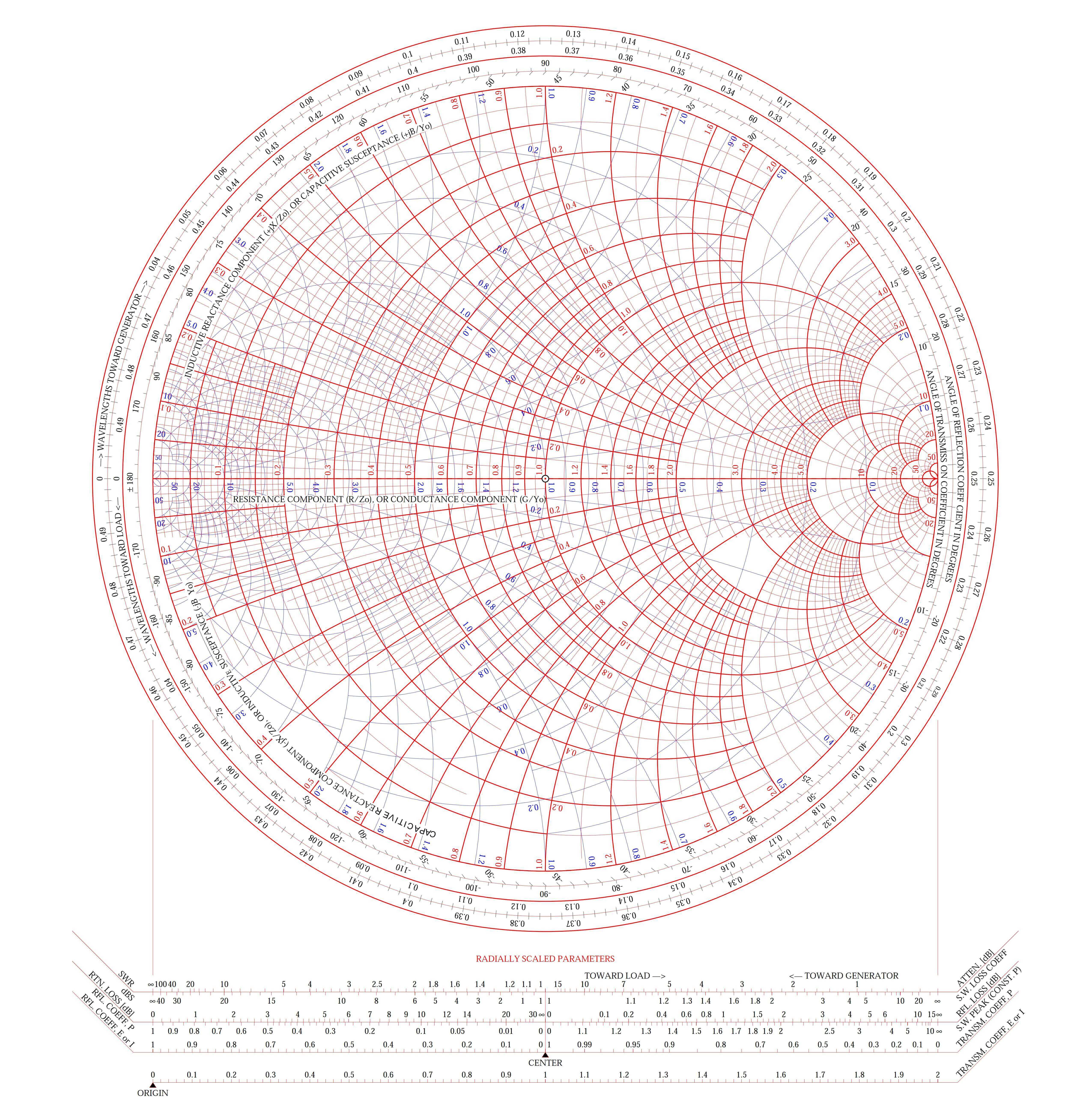
The Smith Chart is a polar plot of complex reflection coefficients (denoted as \(\Gamma\)). This chart simultaneously represents the real and imaginary parts of complex impedance. The real part, denoted as R, ranges from 0 to infinity (\(\infty\)), while the imaginary part, denoted as X, ranges from negative infinity to positive infinity. The Smith Chart can be used to visualize various parameters and functionalities, including but not limited to:
- Complex impedance
- Complex reflection coefficients
- Voltage Standing Wave Ratio (VSWR)
- Transmission line effects
- Designing impedance matching networks
Normalized Impedance
First, we need to convert complex impedance into normalized impedance before plotting it on the Smith Chart. Normalized impedance is calculated by dividing the actual impedance by the system impedance:
In most cases, the system impedance is 50Ω, so essentially, you divide the actual impedance by 50Ω. For example, if the actual impedance is (37+j55)Ω, the normalized impedance is approximately (0.74+j1.10)Ω.
Smith Chart in Detail
On the Smith Chart, the horizontal axis in the middle represents the purely resistive axis (R), where the reactance is always 0. In the region above this axis (R+jX), the impedance is inductive, while in the region below (R-jX), it is capacitive.
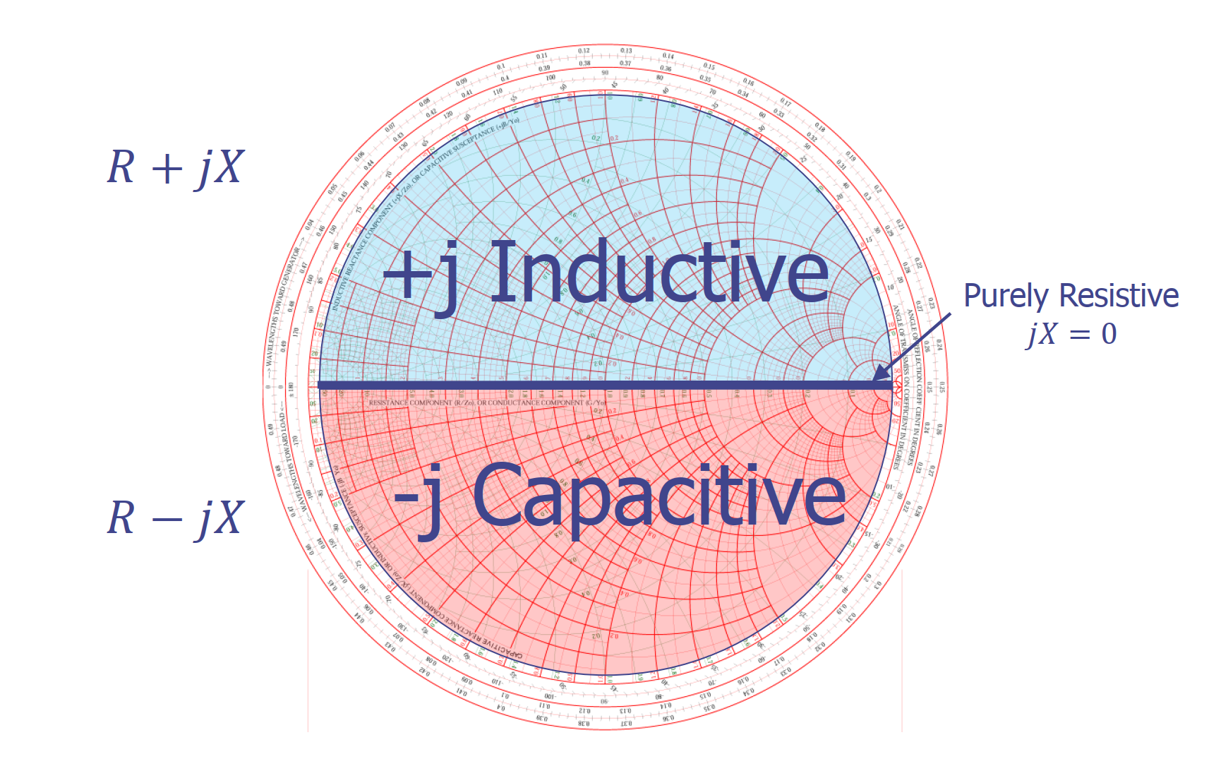
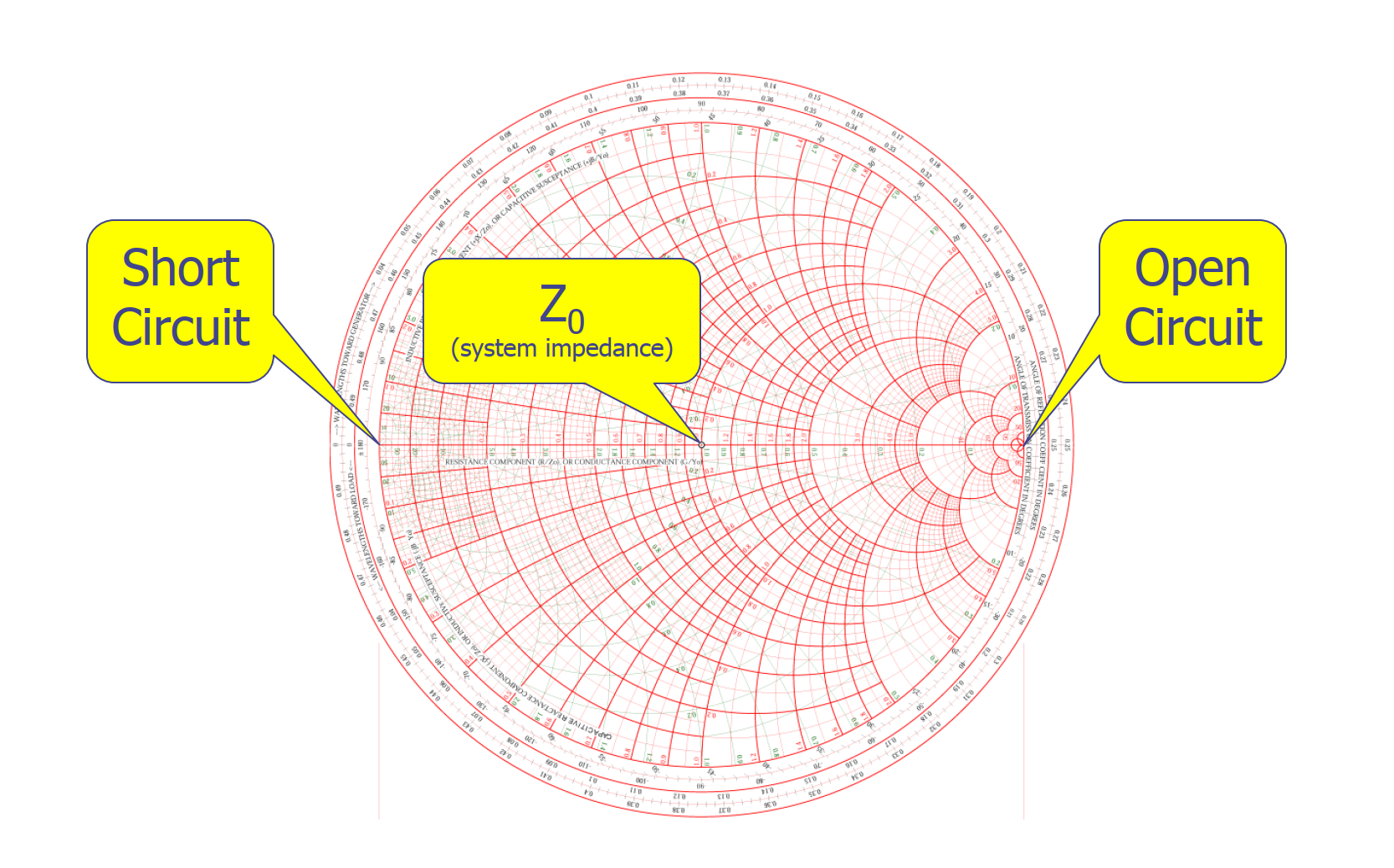
Key Points
There are several key points on the Smith Chart. The central point represents the system impedance (in a 50Ω system, this point corresponds to 50Ω impedance). Along the main axis, the rightmost point represents an open circuit (infinite impedance), and the leftmost point represents a short circuit (0 impedance).
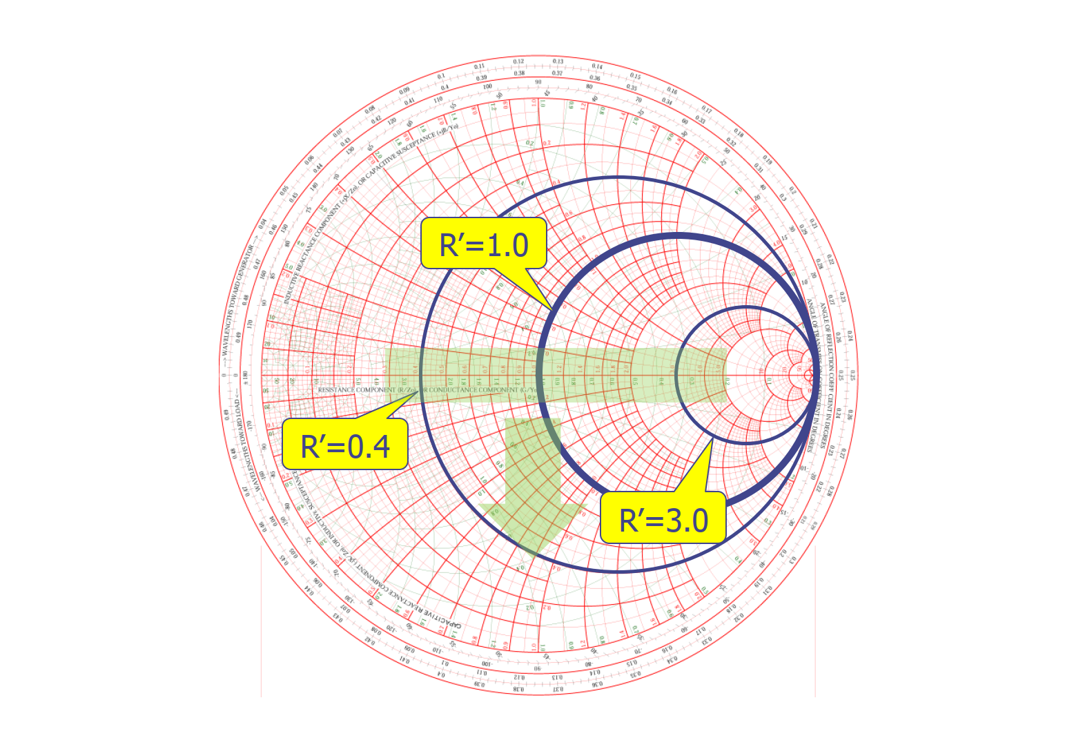
Constant Resistance Circles
On constant resistance circles, the normalized resistance (real part) remains constant. For example, the circle passing through the center has a resistance of 1 (50Ω), indicating that the normalized impedance's real part is 1. In the chart, you can also see constant resistance circles with real parts of 0.4 and 3.0:
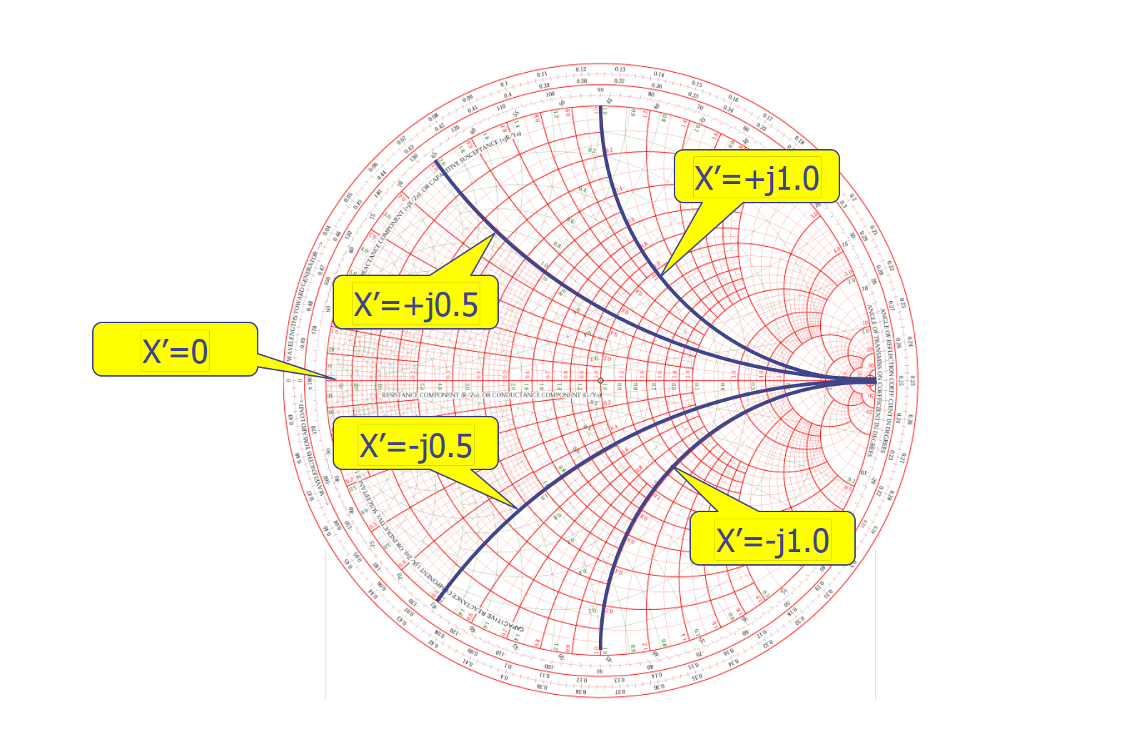
Constant Reactance Arcs
Constant reactance arcs extend from the open-circuit point. The points on these arcs represent the reactance values, i.e., the imaginary part of complex impedance. Larger arc angles indicate greater reactance magnitudes, and as the angle decreases, the reactance magnitude becomes smaller, ultimately reaching 0 (falling on the purely resistive axis, indicating neither inductive nor capacitive behavior). In the chart, you can find constant reactance arcs with reactance values of ±0.5 (imaginary part ±j0.5) and ±1.0 (imaginary part ±j1.0):
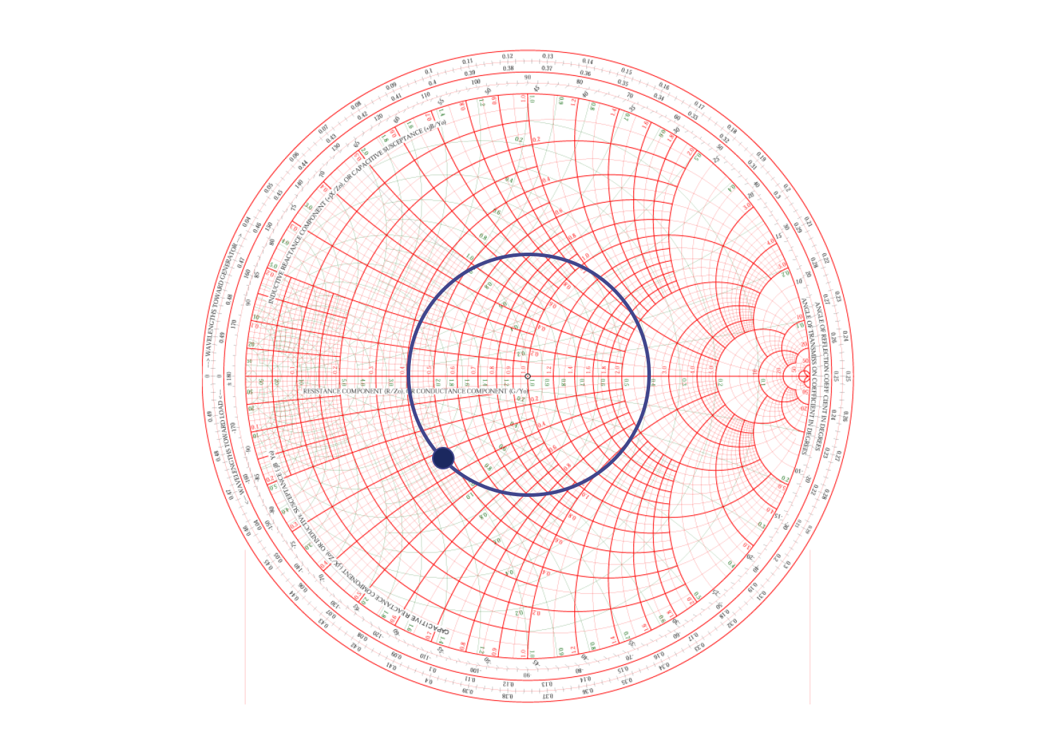
Converting Complex Impedance to Complex Admittance
Admittance (Y) is the reciprocal of impedance, conductance (G) is the reciprocal of resistance, and susceptance (B) is the reciprocal of reactance. When they are complex numbers, calculations can be quite complex. However, on the Smith Chart, you can easily find the corresponding complex admittance value Y' by drawing a circle centered at the origin that passes through the complex impedance point Z'.
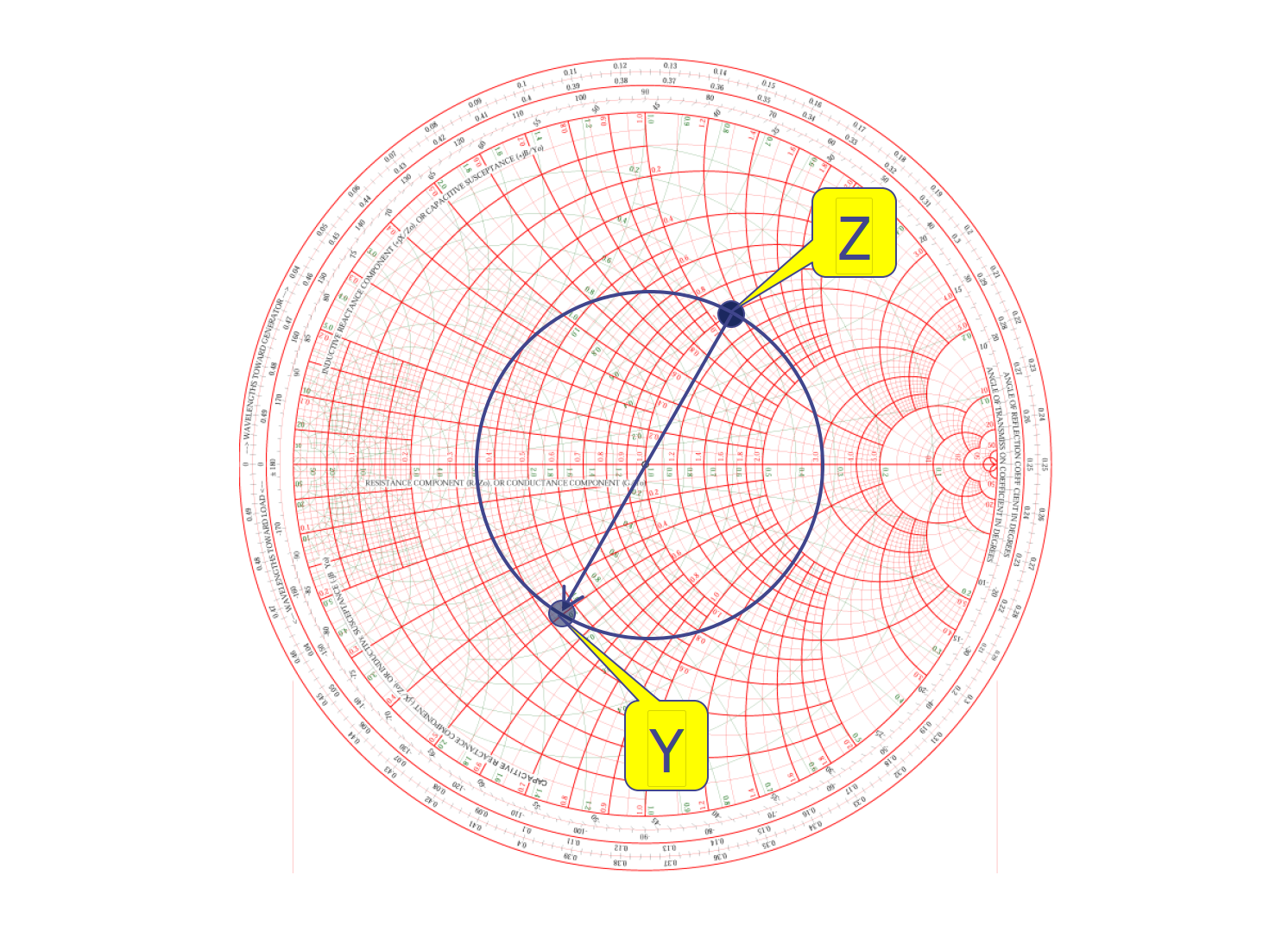
For example, if Z' = 1+j1.1, its corresponding Y' is 0.45-j0.5.
If you have a complex impedance curve, you can rotate the Smith Chart by 180° to obtain the complex admittance curve.
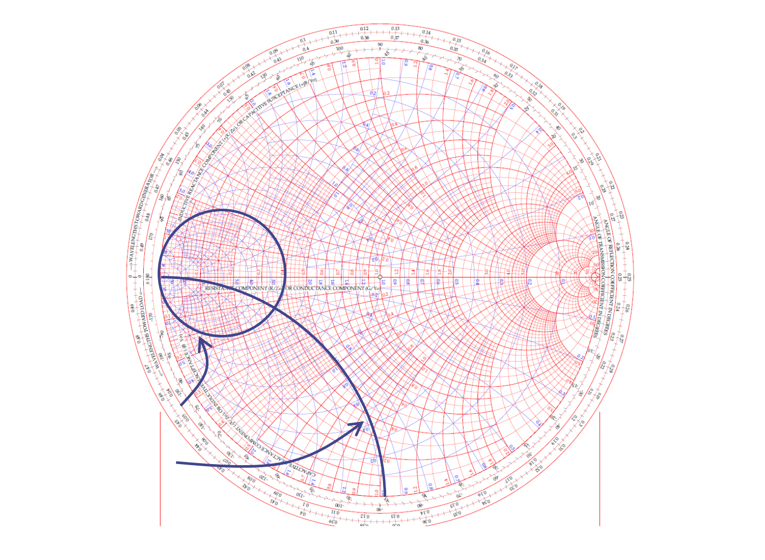
Constant Conductance Circles and Constant Susceptance Arcs
The complete Smith Chart also includes constant conductance circles and constant susceptance arcs, marked in blue in the following image:
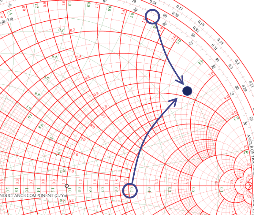
To mark a general value, such as Z=25+j40, on the Smith Chart, start by normalizing it with respect to the 50Ω impedance. Calculate Z' as 0.5+j0.8. You can then locate the circles with R'=0.5 and arcs with X'=0.8, and their intersection point will give you the desired Z':
Radial Scaling Parameters of the Smith Chart
In general, the Smith Chart includes radial scaling parameter axes underneath. Assuming there's a complex impedance point on the chart, connecting it to the center and rotating along the radius to the main axis, projecting it onto the radial scaling parameter axis, as shown in the image below:
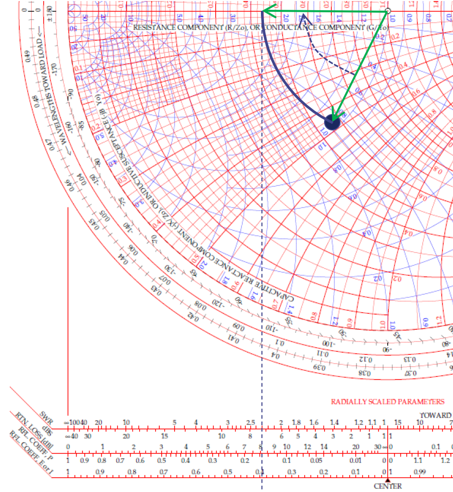
From this axis, you can read several parameters:
- Voltage Standing Wave Ratio (VSWR): 2.3:1
- Return Loss: 8.10dB
- Reflection Coefficient
- Voltage: 0.155
- Power: 0.39
Furthermore, you can observe that the points located on this radius circle have the same parameters.
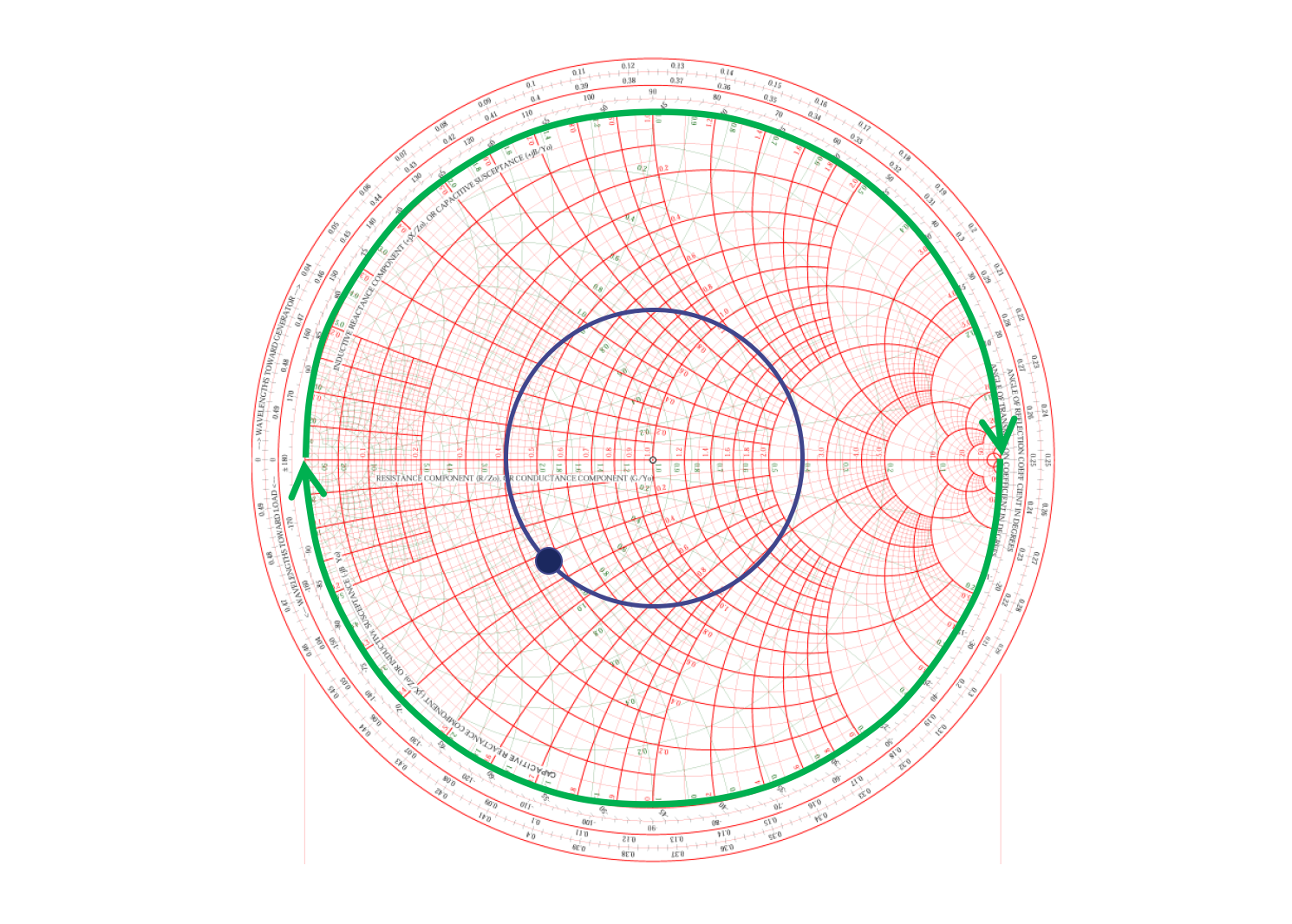
Relationship Between VSWR and Transmission Line
As mentioned earlier, on a circle drawn with the system impedance (center point) as the center and the distance to complex impedance points as the radius, the VSWR of different impedances on the circle is equal. The length of one full rotation around the circle corresponds to half a wavelength. Therefore, as the length of the transmission line from the source to the antenna increases by half a wavelength, the complex impedance will rotate one more time around the circle.
Hence, the length of the transmission line from the source to the antenna should be controlled to be a multiple of half the wavelength of the antenna to ensure that the observed impedance matches the actual impedance of the antenna. If the length is not a multiple of half a wavelength, you can use a transmission line model within SimNEC simulation software to compensate.
There is an interesting phenomenon: if the end of the transmission line is an open circuit and its length is one-fourth of a wavelength (half a rotation), it appears as a short circuit, and vice versa, if the end is a short circuit and its length is one-fourth of a wavelength, the observed characteristics appear as an open circuit.
Design of Matching Circuits
In circuits, we often connect inductors and capacitors in series or parallel to move the complex impedance point and achieve impedance matching.
- Series Inductor: Move clockwise along the constant resistance circle.
- Series Capacitor: Move counterclockwise along the constant resistance circle.
- Parallel Inductor: Move counterclockwise along the constant conductance circle.
- Parallel Capacitor: Move clockwise along the constant conductance circle.
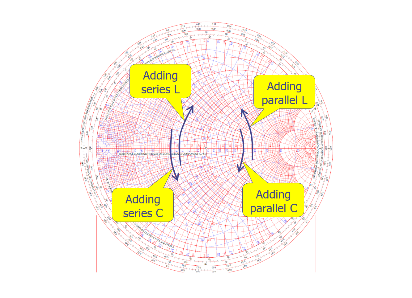
Qualitatively, whether in series or parallel, adding an inductor will move the complex impedance point upwards, while adding a capacitor will move it downwards.
Simple L-Type Matching Circuit
Suppose the measured complex impedance value of the current circuit is \(Z_L\), and you need to adjust it to the ideal $Z_0 (preferably the center point, or secondarily on the 50Ω resistance circle). In that case, you can use inductors or capacitors to create a simple L-shaped matching circuit to move the complex impedance point on the Smith Chart. The choice between inductors and capacitors depends on the initial position of \(Z_L\) on the Smith Chart. Depending on the distribution of \(Z_L\) in the diagram below, you can select the appropriate combination to construct an L-type matching circuit.
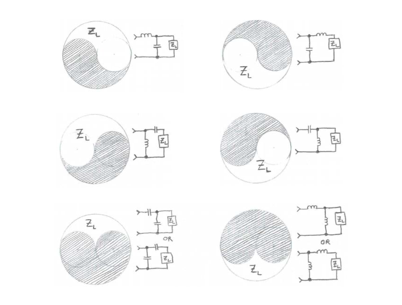
For example, if the initial complex impedance value \(Z_L\) is as shown in the diagram (black dot), you can construct the L-type matching circuit according to the diagram provided to move it to the ideal $Z_0 (red dot):
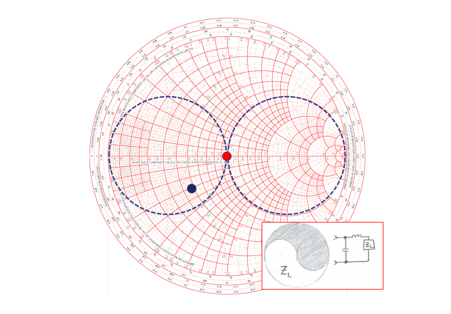
For ease of reference, we've outlined the standard constant conductance and constant resistance circles on the chart. The next steps can be performed using SimNEC simulation software:
- Add series inductance by moving clockwise along the constant resistance circle until it touches the constant conductance circle.
- Add parallel capacitance by moving counterclockwise along the constant conductance circle until it reaches the center point.
The method can be roughly summarized as follows: Start from the vicinity of the load, add the first component to move the complex impedance point onto the standard constant conductance circle or constant resistance circle. Then, add the second component to move it to the center along the standard constant conductance circle or constant resistance circle. The values of the selected components can be read from the software.
For practical tuning of the matching circuit, you can refer to the article Design of General Antenna Matching Circuits.
References and Acknowledgments
- Smith Chart: The History and Significance for RF Designers
- Basics of the Smith Chart - Introduction, Impedance, VSWR, Transmission Lines, Matching
- RF Engineering Basic Concepts: The Smith Chart
Original: https://wiki-power.com/ This post is protected by CC BY-NC-SA 4.0 agreement, should be reproduced with attribution.
This post is translated using ChatGPT, please feedback if any omissions.